User Guide

This comprehensive manual covers all features of the Napari Chromosome Analysis toolkit.

Note

Author: Md Abdul Kader Sagar Affiliation: HITIF/LRBGE/CCR/NCI

Overview

The Napari Chromosome Analysis toolkit is designed for analyzing metaphase chromosomes using advanced image processing techniques. It provides tools for:

• Automated chromosome segmentation using Cellpose

• Multi-channel fluorescence image analysis

• Spot detection for DNA-FISH and CENP-C signals

• Quantitative intensity measurements

• Batch processing capabilities

• Interactive manual correction tools

The Interface

The interface consists of several interactive widgets and buttons, organized as follows:

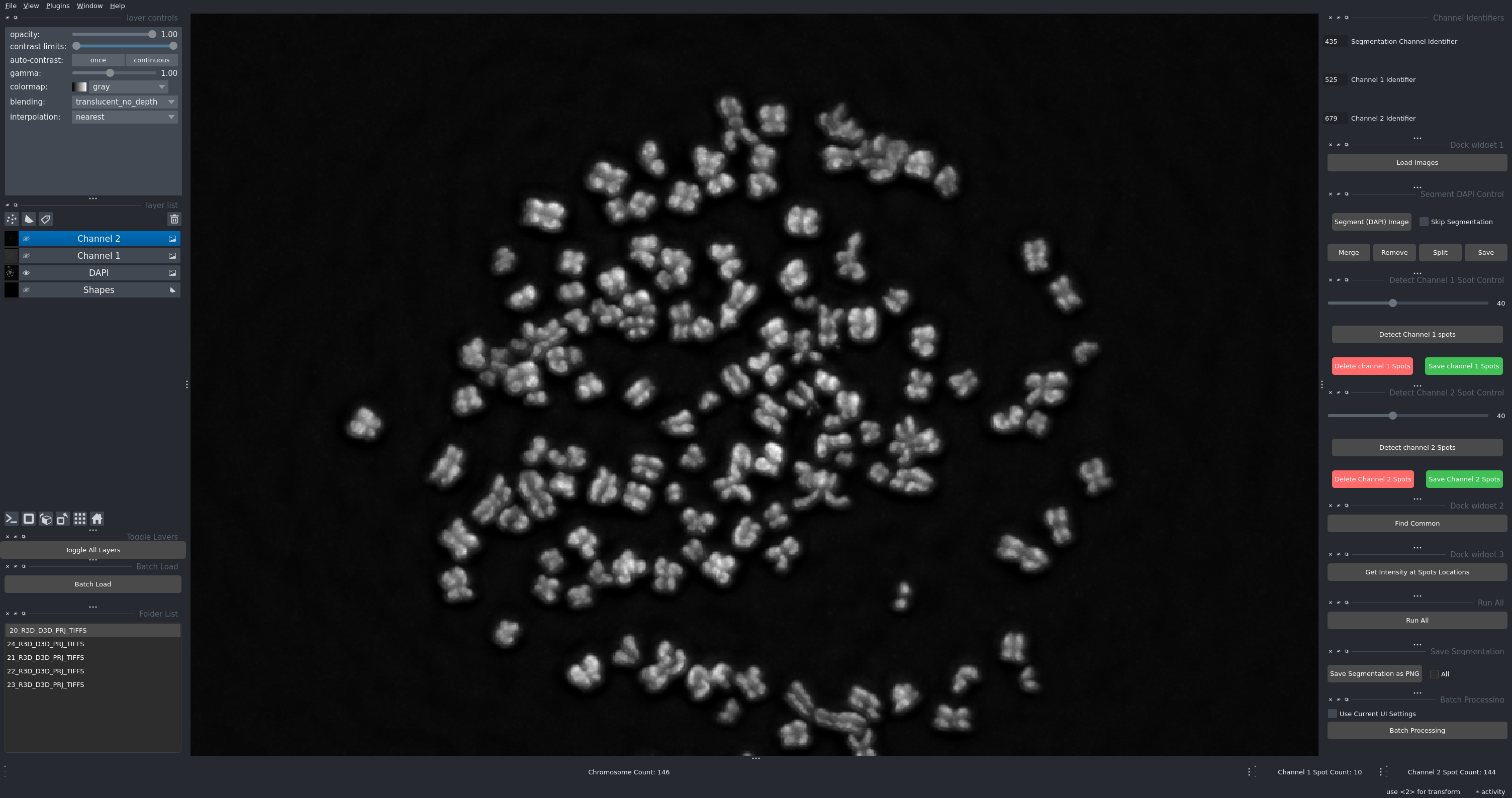
Figure 1: The main interface showing all control panels and the napari viewer.

Main Components:

• Channel Identifiers: Text inputs to specify identifiers for DAPI, DNA-FISH, and CENP-C channels

• Load Images: Button to select a folder containing images

• Segment DAPI Control: Allows segmenting the DAPI image and/or choosing to skip segmentation if needed

• Spot Detection Controls: Adjustable sliders for setting detection thresholds for Channel 1 (DNA-FISH) and Channel 2 (CENP-C)

• Shapes Layer: A layer to draw lines for manual adjustments like merging or removing chromosomes

Step-by-Step Workflow

Step 1: Setting Up Channel Identifiers

Before loading images, you must define the channel identifiers that match your image naming convention:

Channel Identifiers:

• DAPI Channel Identifier: Enter the identifier used for DAPI channel images. For example, 435 if your images are named like R3D_D3D_PRJ_w435.tif

• Channel 1 Identifier: Enter the identifier used for DNA-FISH channel images (e.g., 525)

• Channel 2 Identifier: Enter the identifier used for CENP-C channel images (e.g., 679)

Alternative Naming:

You can also use descriptive identifiers:

• DAPI: dapi

• DNA-FISH: dna_fish

• CENP-C: cenpc

Note

The identifier can appear anywhere in the filename. For example, sample_435_channel.tif or w435.tif will both match the identifier 435.

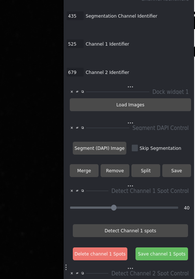
Figure 2: Setting up channel identifiers before loading images.

Step 2: Loading Images

1. Click the Load Images button

2. A file dialog will open - navigate to the folder containing your images

3. Click Select to load the images

4. Notice the left-bottom corner: all folders with images will appear as a list

5. Click any item in the list to load all 3 channels for that image set

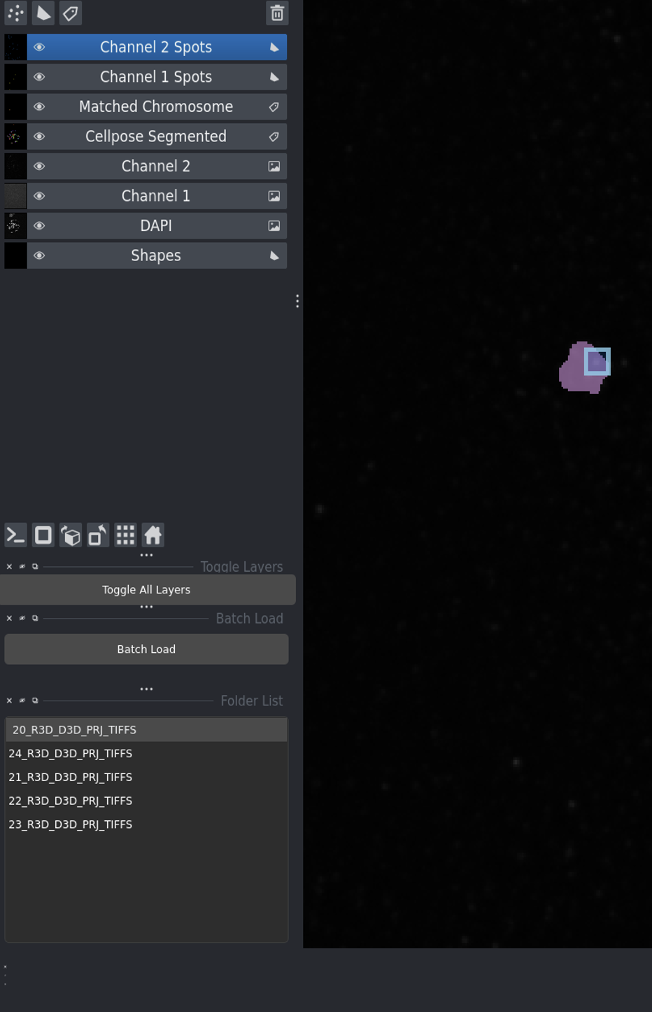
Figure 3: The interface after loading images, showing the folder list and loaded channels.

Tip

If you selected Skip Segmentation, the DAPI image will not be segmented, and spot detection will proceed directly on the other channels.

Understanding the Napari Viewer

After loading images, all 3 channels are visible in the napari viewer:

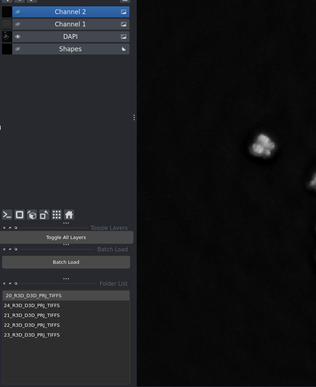
Figure 4: Napari viewer showing all channels and layer controls.

Layer Controls:

• Click the eye icon next to any layer to show/hide that channel

• Use Toggle All Layers to show/hide all layers at once

• Adjust brightness and contrast for each layer individually

• Layers list appears on the left side of the viewer

Step 3: Segmenting DAPI Image

The DAPI segmentation step identifies individual chromosomes using a trained Cellpose model.

1. Click Segment (DAPI) Image

2. The software will process the DAPI channel

3. A new labels layer called “Cellpose Segmented DAPI” will appear in the viewer

4. Each chromosome is assigned a unique label/color

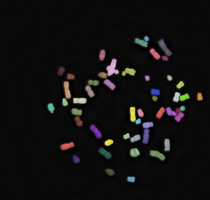
Figure 5: Output of chromosome segmentation showing individual chromosomes labeled with different colors.

Note

If you want to skip segmentation, check the Skip Segmentation checkbox before loading images. This is useful when:

• You don’t have DAPI images

• You only want to analyze DNA-FISH and CENP-C channels

• Chromosomes are not needed for your analysis

Step 4: Adjusting Spot Detection Thresholds

Before detecting spots, adjust the threshold values to optimize detection sensitivity:

DNA-FISH Threshold Slider:

• Range: 0-100 (displayed as 0.0-1.0 internally)

• Lower value = more sensitive (detects more spots, including potential noise)

• Higher value = more selective (detects only bright spots)

CENP-C Threshold Slider:

• Same range and behavior as DNA-FISH

• Optimize based on your image’s signal-to-noise ratio

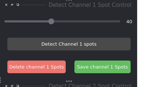
Figure 6: Spot detection threshold sliders for both channels.

Important

Changing the slider resets the spot detection status, requiring you to re-run the spot detection process.

Step 5: Detecting Spots

After setting appropriate thresholds:

1. Click Detect Channel 1 Spots to identify spots in the DNA-FISH image

2. Click Detect Channel 2 Spots for the CENP-C image

3. Detected spots will be displayed as labels in the napari viewer

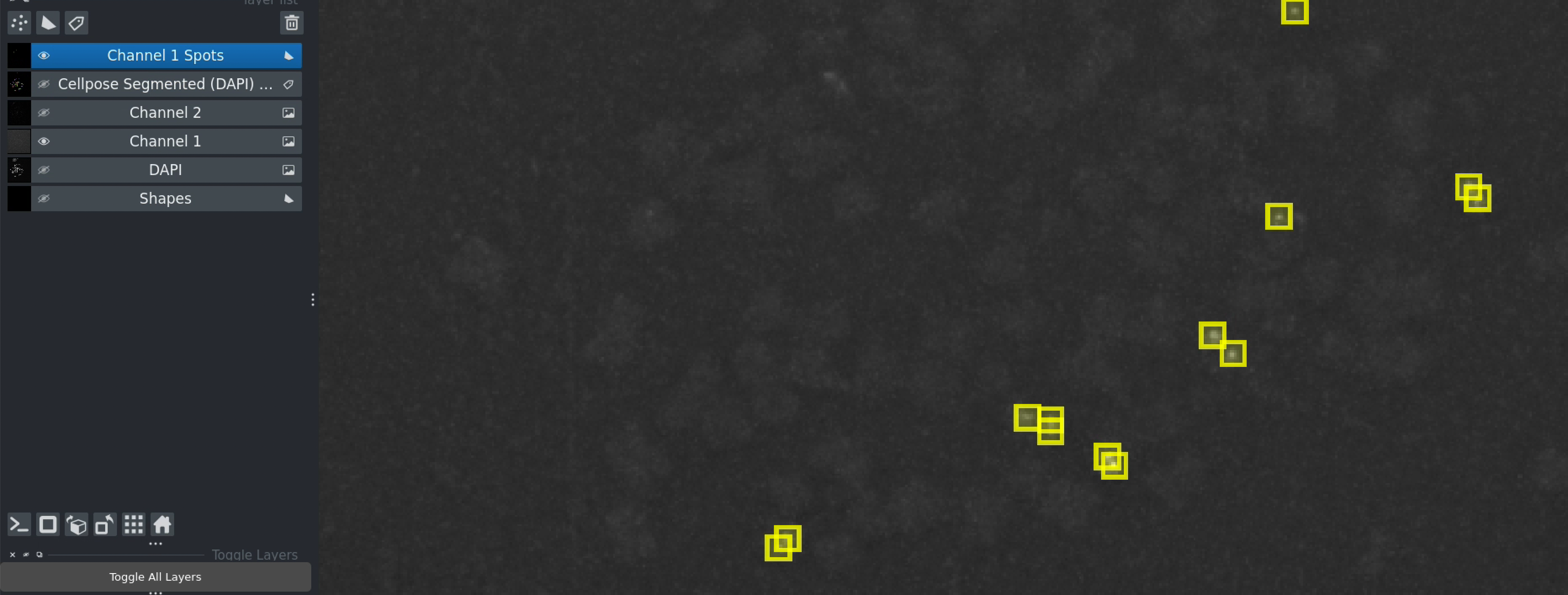
Figure 7: After clicking “Detect Channel 1 Spots” - a new layer shows detected spots as brown markers.

Viewing Detected Spots:

• A new layer “Channel 1 spots” appears for DNA-FISH

• Brown/colored markers indicate detected spot locations

• Toggle the DNA-FISH channel visibility to see how spots overlay with the signal

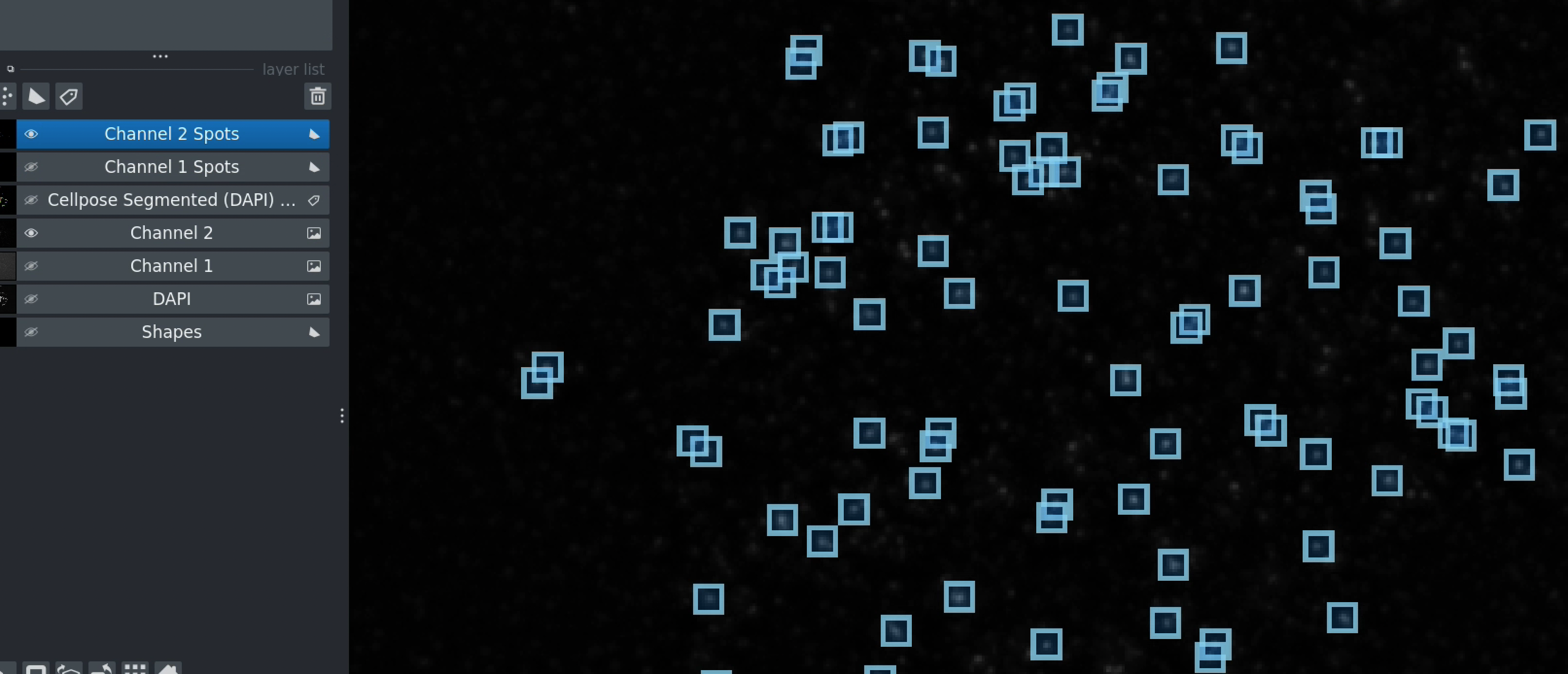
Figure 8: Both channels showing detected spots after processing Channel 2.

Tip

If you already ran spot detection and want to redo it:

1. Adjust the threshold slider (even slightly)

2. Click the detection button again

Step 6: Finding Common Chromosomes

This step identifies chromosomes where both DNA-FISH and CENP-C signals are present:

1. Click Find Common

2. The software identifies matching regions between both channels

3. Common labels are overlaid, highlighting areas where both signals co-localize

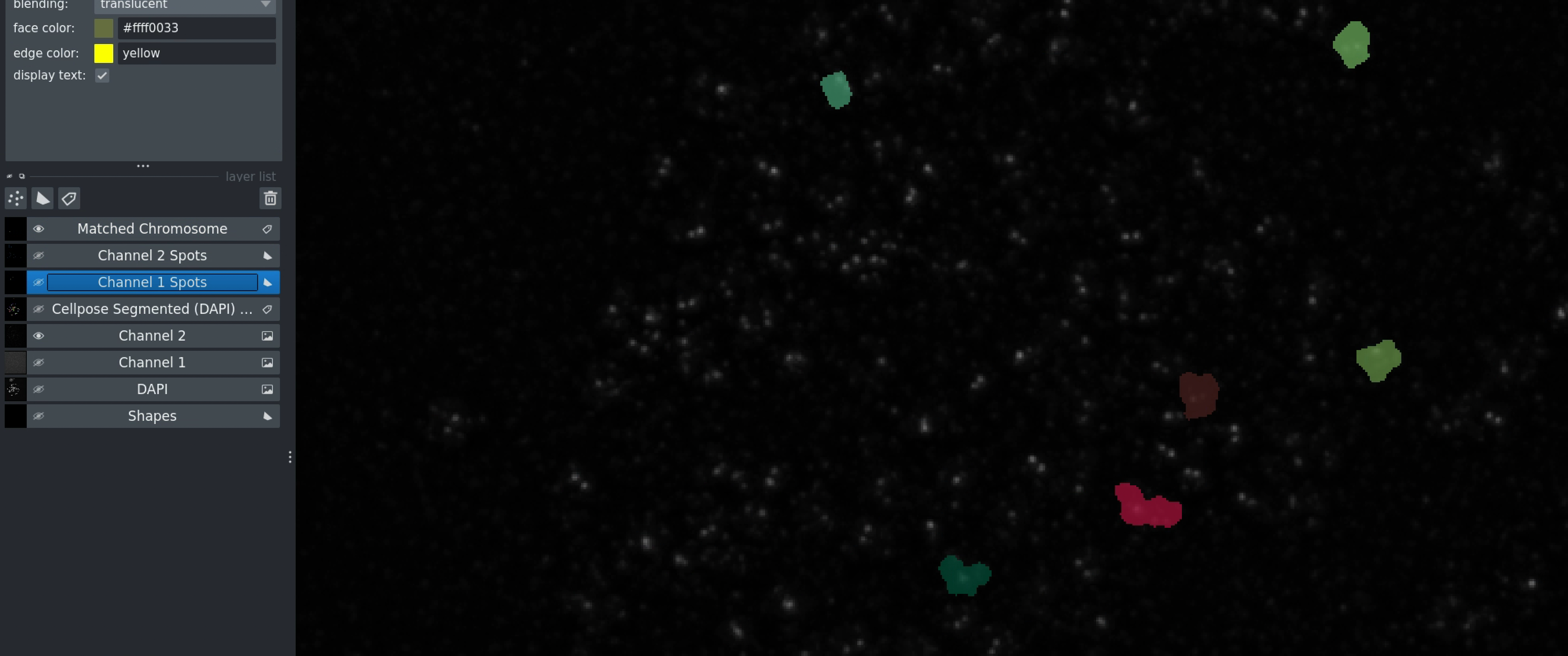
Figure 9: Interface for finding common regions between channels.

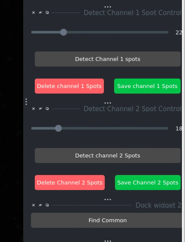
Figure 10: Visualization of common regions where both signals overlap.

This step is crucial for:

• Filtering out background noise

• Ensuring both signals are present in the analysis region

• Improving measurement accuracy

Step 7: Calculating Intensity and Exporting Results

The final analysis step measures signal intensities at spot locations:

1. Click Get Intensity at Spots Location

2. The software calculates:

   • Channel 2 intensity at Channel 1 spot locations

   • Channel 1 intensity at Channel 2 spot locations

3. A CSV file is automatically saved in the same folder as your images

4. Filename format: <folder_name>_intensity.csv

Locating Your Results:

Check the terminal window to see where the file is being saved.

CSV File Contents:

The exported CSV contains:

• Spot coordinates (X, Y)

• Intensity values for both channels

• Metadata (folder name, parameters used)

Analysis Without Segmentation

For cases where chromosome segmentation is not needed:

When to Use:

• No DAPI images available

• Only interested in DNA-FISH and CENP-C co-localization

• Analyzing entire image without chromosome boundaries

How to Use:

1. Check Skip Segmentation before loading images

2. Load only DNA-FISH and CENP-C channels (DAPI is ignored even if present)

3. Follow Steps 4-7 normally (spot detection, finding common regions, intensity calculation)

Analysis Approach:

• Intensity is calculated at DNA-FISH spots from the CENP-C channel

• No chromosome boundaries are used

• Everything else remains the same

Automated Analysis

Run All

The Run All button automates the entire workflow:

1. Check/uncheck Skip Segmentation as per your requirement

2. Adjust threshold sliders to desired values

3. Click Run All

The software will automatically execute:

• Segmentation (if not skipped)

• Channel 1 spot detection

• Channel 2 spot detection

• Find common regions

• Calculate and export intensities

Figure 11: The “Run All” button for automated processing.

Tip

Use “Run All” when you’ve established optimal thresholds and want to quickly process individual images.

Batch Processing

For processing multiple image folders with consistent settings:

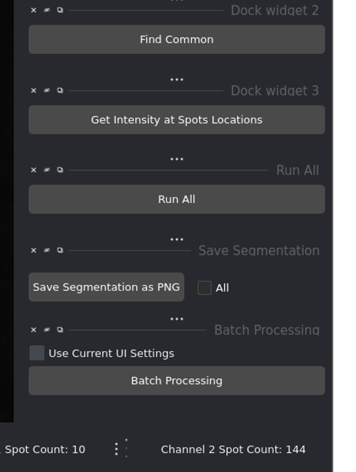
Figure 12: Batch processing controls for analyzing multiple image sets.

How Batch Processing Works:

1. Load all folders using the folder list on the left

2. Configure your settings (thresholds, segmentation options)

3. Choose your processing mode:

   • Use Current UI Settings (checked): Recalculates everything from scratch using the same thresholds for every image

   • Use Current UI Settings (unchecked): Uses previously saved settings for each image folder

4. Click Batch Processing

Output:

• Individual CSV files saved in each image folder

• Summary CSV file created in the root directory

• Consolidated results for all processed images

Note

Batch processing goes through all opened files in the list view and calculates necessary intensity measurements for each.

Manual Correction Tools

Step 8: Merging Chromosomes

When segmentation incorrectly separates a single chromosome into multiple regions:

Procedure:

1. Select the Shapes layer from the layer list (lower left corner)

2. Select the Polygon/Draw tool from the top toolbar (marked with a pencil icon)

3. Draw a line connecting the chromosome regions you want to merge:

   • Click on the first segmented chromosome

   • Continue drawing the line over to the second chromosome

   • Double-click to finish drawing

4. Click Merge Chromosomes

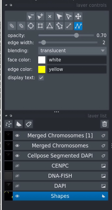
Figure 13: Drawing a line to indicate chromosomes to merge.

Important Steps:

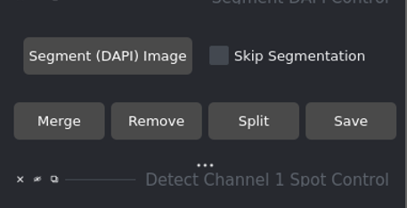
Figure 14: Make sure both the segmented layer and shapes layer are visible.

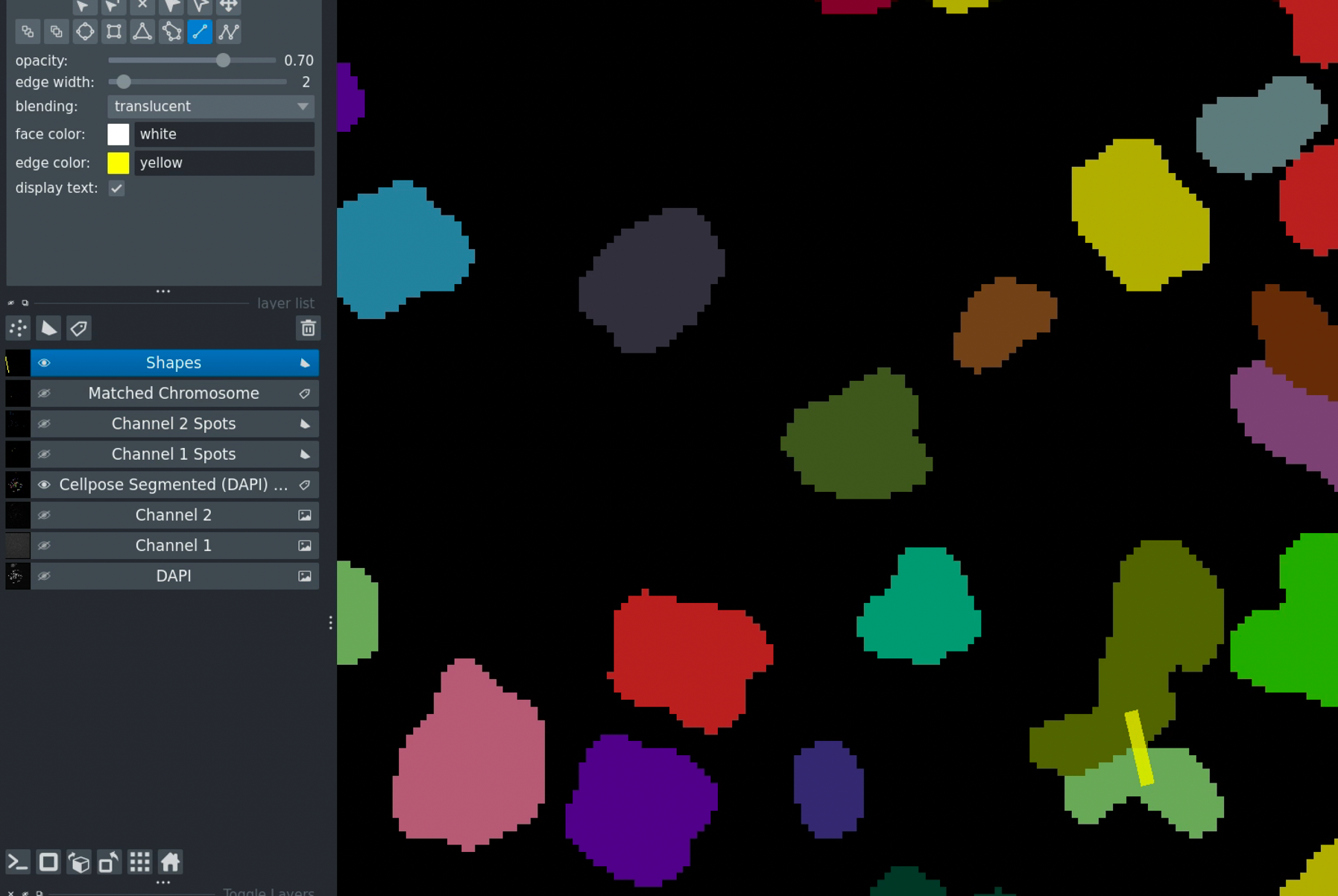
Figure 15: Ensure the shapes layer is selected when drawing.

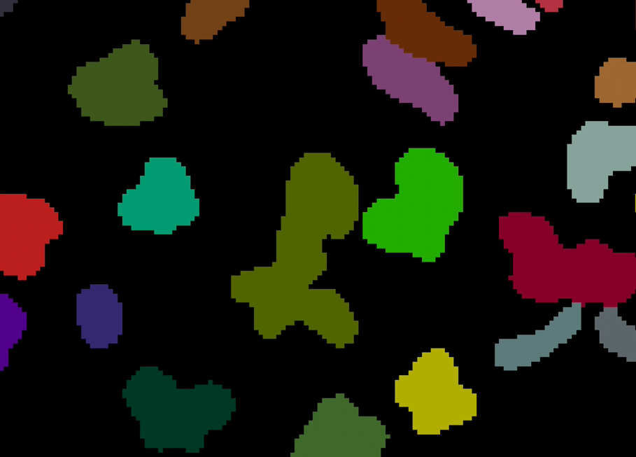
Figure 16: Result after clicking “Merge Chromosomes” - the regions are now combined.

Removing Chromosomes

To delete unwanted chromosomes from the analysis:

Procedure:

1. Select the Shapes layer

2. Draw a line through the chromosome you want to remove

3. Click Remove

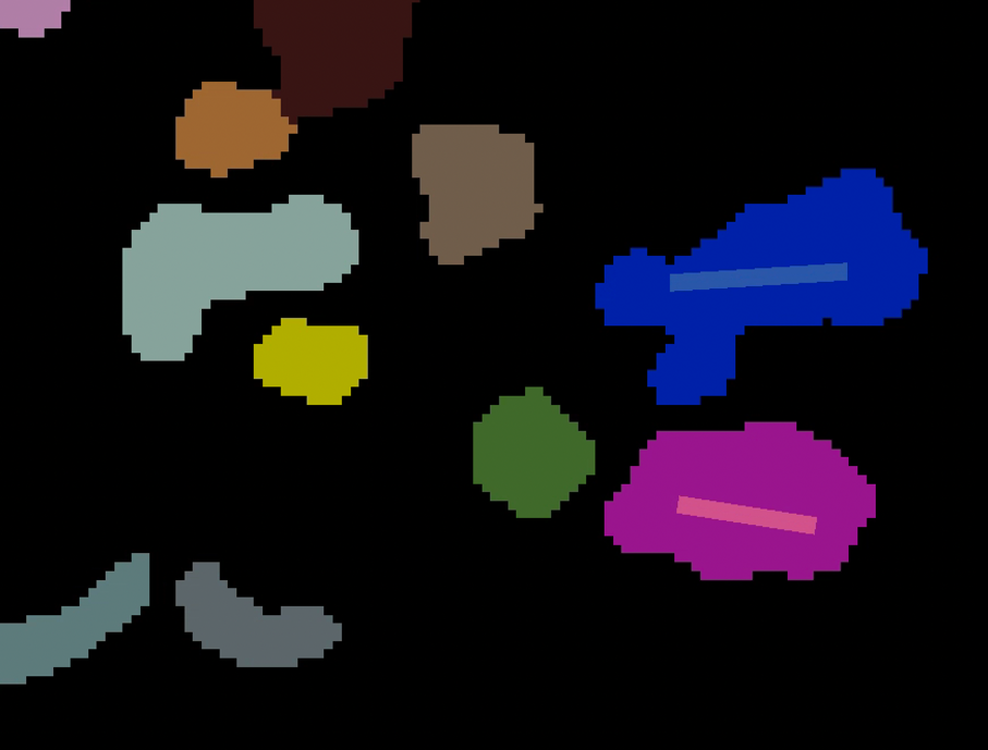
Figure 17: Drawing over a chromosome to mark it for removal.

Result:

Figure 18: The updated chromosome layer excluding the removed chromosome.

Saving Manual Corrections

After making manual corrections:

1. Click Save in the interface

2. Your corrections are stored

3. Next time you load this image set, it will use the updated segmentation

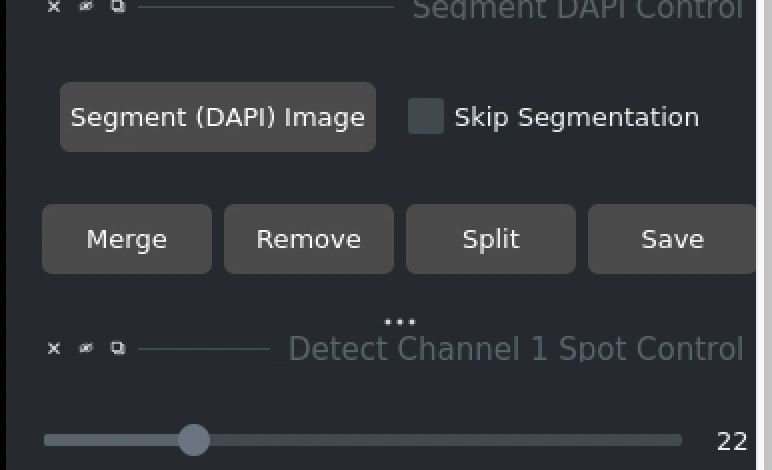
Figure 19: Save your work to preserve manual corrections.

Updating Spot Detection

You can also manually correct spot detections:

Deleting Channel 1 Spots:

1. Select the Shapes layer

2. Draw shapes (squares or polygons) over spots you want to delete

3. Click Delete Channel 1 Spots

4. The spots layer will be updated

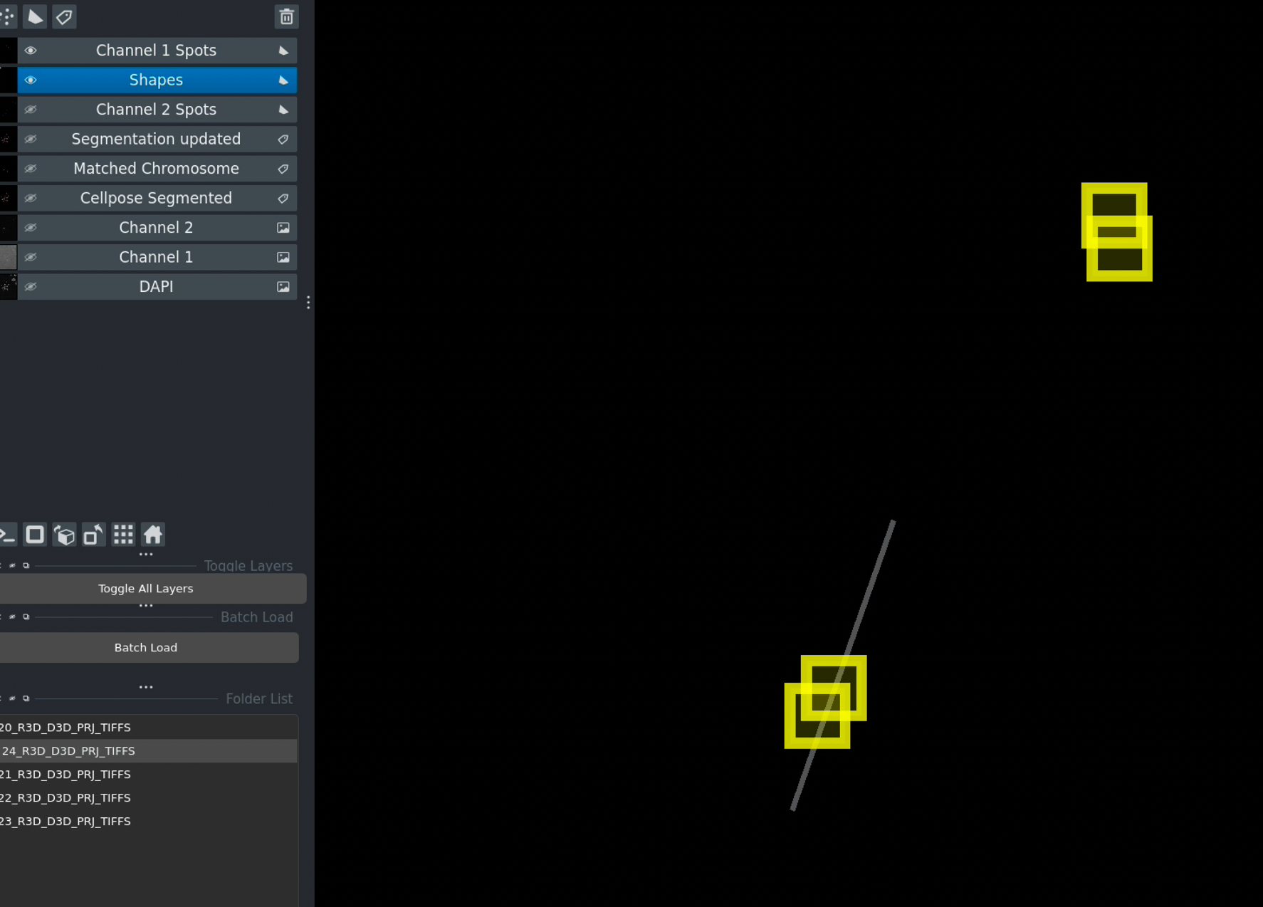
Figure 20: Drawing shapes to mark spots for deletion.

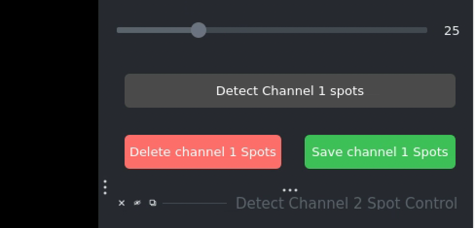
Figure 21: Updated spot layer after deletion.

Deleting Channel 2 Spots:

The same process applies to Channel 2:

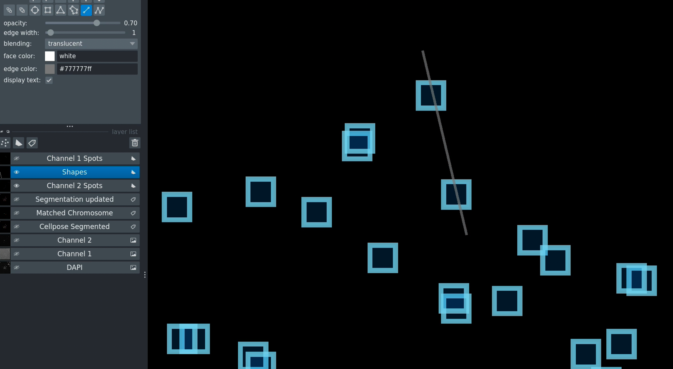
Figure 22: Interface for deleting Channel 2 spots.

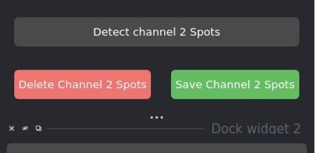
Figure 23: Updated Channel 2 spots after manual correction.

Important

• Make sure the shapes layer is selected when drawing

• Click Save to keep your spot corrections

• Without saving, the software will use default detected spots when you reload

Data Export and Saving

Saving Results

Processed Images:

• All visualizations (segmented images, detected spots) remain in the napari viewer

• Use napari’s export options: File → Save Selected Layer(s)

• Export individual layers as PNG or TIFF

Intensity Data:

• CSV files with intensity data are saved automatically

• Location: Same folder as the analyzed images

• Filename: <folder_name>_intensity.csv

Exporting Specific Layers:

1. Select the layer you want to export

2. Navigate to File → Save Selected Layer(s) in the napari menu

3. Choose format and location

Image Requirements

Supported Formats:

• TIFF (recommended for multi-channel microscopy)

• PNG

• JPG

Channel Requirements:

The software expects multi-channel fluorescence microscopy images with:

• DAPI channel: For chromosome segmentation

• DNA-FISH channel: For detecting specific DNA sequences

• CENP-C channel: For detecting centromere proteins

File Naming Conventions:

Use consistent identifiers in filenames. Examples:

• sample_001_w435.tif (DAPI)

• sample_001_w525.tif (DNA-FISH)

• sample_001_w679.tif (CENP-C)

Or:

• cell1_dapi.tif

• cell1_dna_fish.tif

• cell1_cenpc.tif

Parameters and Settings

Detection Thresholds

DNA-FISH Threshold:

• Range: 0-100% (displayed as 0.0-1.0 internally)

• Lower values = more sensitive detection

• Higher values = more specific detection

CENP-C Threshold:

• Same range and behavior as DNA-FISH

• Optimize based on signal-to-noise ratio

• Test on sample images before batch processing

Segmentation Parameters

Cellpose Settings:

• Model: Custom trained model for metaphase chromosomes

• Diameter: Automatically determined by the model

• Channels: [0,0] for grayscale DAPI input

• GPU acceleration: Enabled by default (if available)

Post-processing Options:

• Remove small objects: Filters out noise and artifacts

• Remove edge objects: Excludes chromosomes touching image borders

• Fill holes: Fills gaps within chromosome regions

• Smooth boundaries: Applies morphological smoothing

Error Handling & Tips

Common Error Messages

“No images found”

• Check folder structure

• Verify file naming conventions match your identifiers

• Ensure images are in supported formats

“CUDA out of memory”

• Reduce image size

• Use CPU mode instead of GPU

• Close other GPU-intensive applications

“Model not found”

• Verify Cellpose model path in code

• Ensure the trained model file is accessible

Troubleshooting

Segmentation Problems:

• Check DAPI image quality and contrast

• Verify that chromosomes are well-separated in the image

• Adjust post-processing parameters

• Use manual correction tools if needed

Spot Detection Issues:

• Optimize threshold values using test images

• Check for proper image focus

• Review channel assignments

• Ensure proper background subtraction

Performance Issues:

• Enable GPU acceleration for Cellpose

• Reduce image size if memory limited

• Process smaller batches

• Close unnecessary applications

File Loading Errors:

• Verify file naming conventions

• Check image formats (TIFF preferred for microscopy)

• Ensure all required channels are present

• Check file permissions

Best Practices

Image Acquisition

• Use consistent imaging parameters across all samples

• Ensure proper focus across all channels

• Optimize exposure times for each channel to avoid saturation

• Maintain consistent sample preparation protocols

Data Organization

• Use clear, hierarchical folder structures

• Follow consistent naming conventions

• Keep raw and processed data separate

• Document analysis parameters for reproducibility

Quality Control

• Manually review a subset of results

• Check for systematic errors in segmentation or detection

• Validate thresholds on test images before batch processing

• Compare automated results with manual counts when possible

Parameter Optimization

• Test different threshold values on representative images

• Document optimal parameters for different imaging conditions

• Use the same parameters for samples that should be compared

• Re-optimize if imaging conditions change

Performance Optimization

• Use GPU acceleration when available

• Process similar images in batches

• Optimize threshold values beforehand to minimize re-processing

• Clean up intermediate files regularly to save disk space

Data Backup

• Regularly backup raw data

• Save analysis parameters with results

• Keep multiple versions of processed data if needed

• Document any manual corrections made

Summary

This user guide has covered:

• Complete step-by-step workflow from loading to analysis

• Manual correction tools for quality control

• Batch processing for high-throughput analysis

• Troubleshooting common issues

• Best practices for optimal results

For API reference and programmatic usage, see API Documentation.

For installation instructions, see Installation.

Contact

For questions, issues, or support:

• Email: sagarm2@nih.gov

• Affiliation: HITIF/LRBGE/CCR/NCI